Silicon
Crystalline silicon is a well studied prototypical material that due to its simple cubic crystalline structure becomes very suitable as a working example.
Preparations
In order to calculate the anharmonic effects fist it is necessary to define the unit cell in a VASP POSCAR type file:
 Si
   1.00000000000000
     5.4365330000000000    0.0000000000000000    0.0000000000000000
     0.0000000000000000    5.4365330000000000    0.0000000000000000
     0.0000000000000000    0.0000000000000000    5.4365330000000000
   Si
     8
Direct
  0.8750000000000000  0.8750000000000000  0.8750000000000000
  0.8750000000000000  0.3750000000000000  0.3750000000000000
  0.3750000000000000  0.8750000000000000  0.3750000000000000
  0.3750000000000000  0.3750000000000000  0.8750000000000000
  0.1250000000000000  0.1250000000000000  0.1250000000000000
  0.1250000000000000  0.6250000000000000  0.6250000000000000
  0.6250000000000000  0.1250000000000000  0.6250000000000000
  0.6250000000000000  0.6250000000000000  0.1250000000000000
Using Phonopy the harmonic forces can be calculated as detailed in phonopy online tutorial. During the calculation, a SPOSCAR file which contains a super cell of the original POSCAR file is generated. This file can be used to calculate the MD in VASP.
Note: The super cell used in Phonopy to calculate the harmonic forces and the one used to calculate the MD in VASP can be different. Phonopy can easly generate a super cell with the desired size using the command:
$ phonopy -d --dim="2 2 2" -c POSCAR_unitcell
This generates a SPOSCAR file containing a 2x2x2 super cell of POSCAR_unitcell file. Alternativelly, DynaPhoPy can also be used to generate a super cell in VASP POSCAR format using the command:
$ dynaphopy input_file --dim 2 2 2 -c_poscar SPOSCAR
input_file is a plain text file contains the information of which unitcell is used to build the super cell. This is a short example of the contains of this file (other keywords may be included):
STRUCTURE FILE POSCAR
/home/user/Si-phonopy/POSCAR_unitcell
This file can also be empty, in this case DynaPhoPy will use a POSCAR named file placed in the work directory as unit cell, but input_file should exist.
Warning: You may need to update numpy if this command fails
VASP MD calculation is carried out using the generated super cell and defining a regular VASP MD input like this example:
      PREC = Normal                  # Precision
    IBRION = 0
      ISYM = 0                       # Disable symmetry
     SMASS = 0                       # Define Thermostat
    MDALGO = 2                       # Nose Hoover thermostat
     POTIM = 0.7                     # Step length
     TEBEG = 800                     # Temperature
       NSW = 200000                  # Number of time steps
    NELMIN = 2
      NELM = 100
     ENCUT = 300
     EDIFF = 1.000000e-06            # Energy precision
    ISMEAR = 0
     SIGMA = 0.01
     IALGO = 38
       GGA = PS
     LREAL = .TRUE.
   ADDGRID = .TRUE.
     LWAVE = .FALSE.
    LCHARG = .FALSE.
EDIFF may have great influence in the exactitute of the results. Longer time step lenghts are recomended to increase the convergence of phonon linewidths but to long could compromise the reliability of the simulation.
Once VASP XDATCAR and Phonopy FORCE_CONSTANTS are generated the only thing left needed to run DynaPhoPY is a DynaPhoPy input.
STRUCTURE FILE POSCAR
/home/user/Si-phonopy/POSCAR_unitcell

FORCE CONSTANTS
/home/user/Si-phonopy/FORCE_CONSTANTS

PRIMITIVE MATRIX
0.0 0.5 0.5
0.5 0.0 0.5
0.5 0.5 0.0

SUPERCELL MATRIX PHONOPY
2 0 0
0 2 0
0 0 2

BANDS
0.0,   0.0,   0.0         0.5,   0.0,  0.5
0.5,   0.0,   0.5         0.625  0.25  0.625
0.375, 0.375, 0.75        0.0,   0.0,  0.0
0.0,   0.0,   0.0         0.5,   0.5,  0.5
Note: there is no restriction in the input file about the number of blank lines between options. Comments are also allowed. All options are optative and can be omitted to use the default value
At this point all the information needed to run Dynaphopy is complete
Calculation examples
- Plot wave vector projection power spectrum at L point from 0 to 16 THz (200 samples) using last 500000 time steps in XDATCAR file:
$ dynaphopy input_file XDATCAR -n 500000 -ts 0.0007 -pw -q 0.5 0.5 0.5 -r 0 16 200
- Save phonon mode projection power spectrum at X point (0.5 0 0.5) to spectrum.dat file using lasts 80000 times teps:
$ dynaphopy input_file XDATCAR -n 80000 -ts 0.0007 -sw spectrum.dat -q 0.5 0.0 0.5
#  frequency	     phonon1    	    phonon2		     phonon3
    0.0000	1.6287598014e-01	1.2511061132e-01	3.4403852187e-03	2.3601374123e-03	2.8351033106e-03	2.4230063427e-03
    0.0025	1.6287848353e-01	1.2511254847e-01	3.4404392354e-03	2.3601725698e-03	2.8351431247e-03	2.4230438285e-03
    0.0050	1.6288599372e-01	1.2511834502e-01	3.4406010527e-03	2.3602771107e-03	2.8352621011e-03	2.4231555872e-03
    0.0075	1.6289848089e-01	1.2512798607e-01	3.4408711363e-03	2.3604519665e-03	2.8354602400e-03	2.4233420845e-03
    0.0100	1.6291600466e-01	1.2514150143e-01	3.4412494861e-03	2.3606969044e-03	2.8357380070e-03	2.4236030877e-03
    0.0125	1.6293852031e-01	1.2515886128e-01	3.4417354036e-03	2.3610112257e-03	2.8360949364e-03	2.4239385966e-03
    .....	................	................	................	................	2.8365314938e-03	2.4243488442e-03
- Peak analysis at Γ point using MEM method (parallel) with 1000 coeficients:
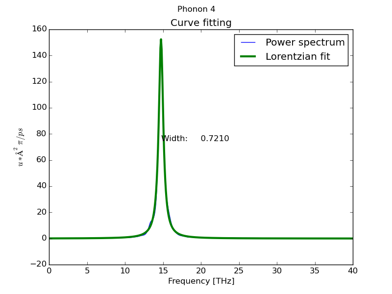
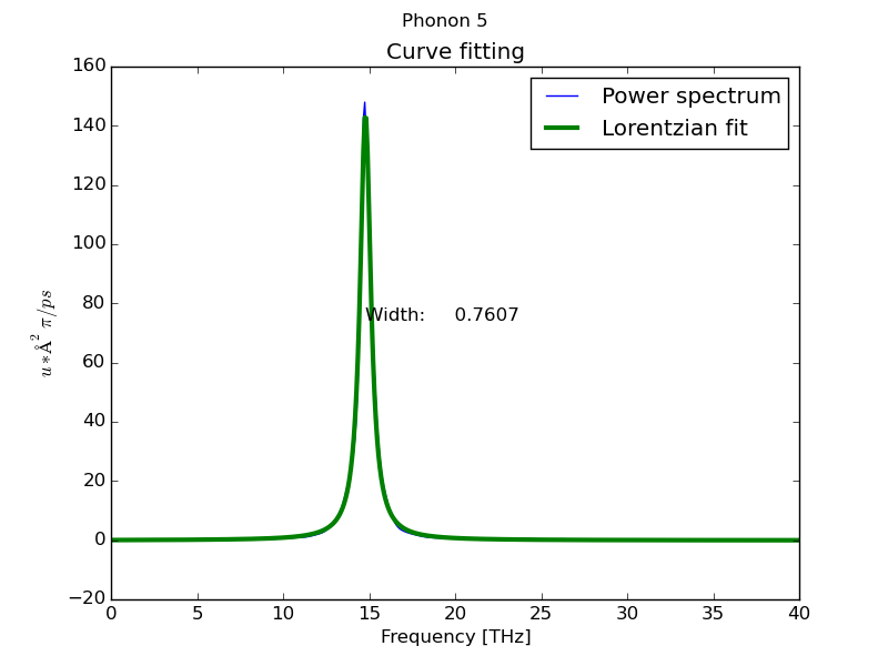
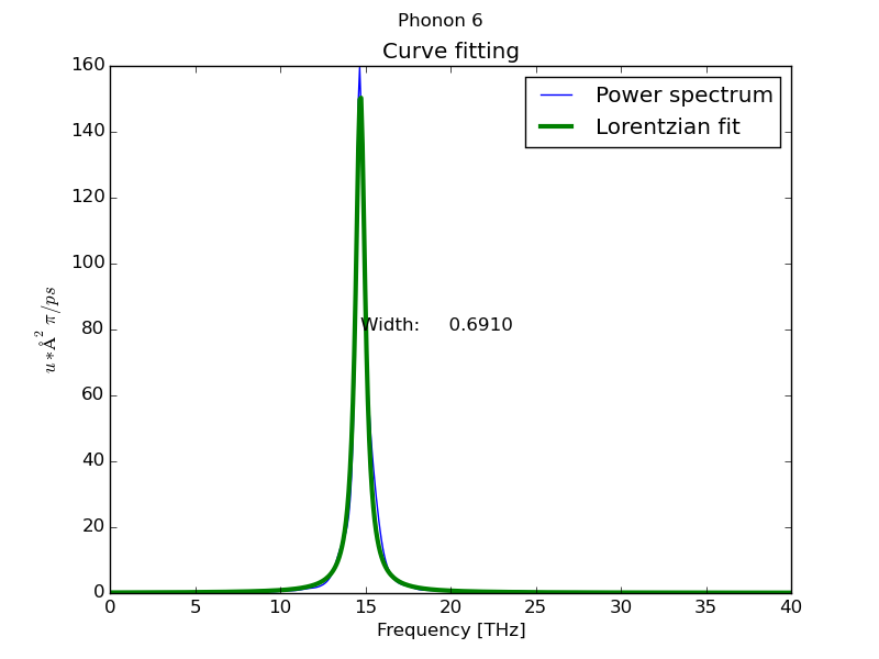
$ dynaphopy input_file XDATCAR -n 5000000 -ts 0.0007 -pa -psm 4 -cf 1000
Peak # 4
----------------------------------------------
Width                             0.336054 THz
Position                         14.591885 THz
Area (<K>)    (Lorentzian)        0.030740 eV
Area (<K>)    (Total)             0.033473 eV
<|dQ/dt|^2>                       0.061479 eV
Occupation number                 5.901073
Fit temperature                 711.985996 K
Base line                         0.000072 eV * ps
Maximum height                    0.058233 eV * ps
Fitting global error              0.014987
Frequency shift                  -0.544369 THz

Peak # 5
----------------------------------------------
Width                             0.336054 THz
Position                         14.591885 THz
Area (<K>)    (Lorentzian)        0.030740 eV
Area (<K>)    (Total)             0.033473 eV
<|dQ/dt|^2>                       0.061479 eV
Occupation number                 5.901073
Fit temperature                 711.985996 K
Base line                         0.000072 eV * ps
Maximum height                    0.058233 eV * ps
Fitting global error              0.014987
Frequency shift                  -0.544369 THz

Peak # 6
----------------------------------------------
Width                             0.336054 THz
Position                         14.591885 THz
Area (<K>)    (Lorentzian)        0.030740 eV
Area (<K>)    (Total)             0.033473 eV
<|dQ/dt|^2>                       0.061479 eV
Occupation number                 5.901073
Fit temperature                 711.985996 K
Base line                         0.000072 eV * ps
Maximum height                    0.058233 eV * ps
Fitting global error              0.014987
Frequency shift                  -0.544369 THz


- Load interactive interface from hdf5 file:
$ dynaphopy input_file -lv velocity_800.h5 -n 50000 -i
- Harmonic eigenvectors representation
- Boltzmann analysis
Maxwell-Boltzmann distribution analysis
----------------------------------------------
Average: 4.0741982e+01 Angstrom/ps
Deviation: 1.7195930e+01 Angstrom/ps
Distribution parameter: 2.5531721e+01 Angstrom/ps
Temperature fit: 788.818186 K
- Renormalized phonon bands
LAMMPS calculations
LAMMPS input preparation can be a little tricky, since is not possible to automatically generate the simulations cell using create_atoms command. In order to keep consistency with Phonopy calculation and DynaPhoPy the cell has to be defined manually to preserve the same order of atoms. To do this, it is convenient to prepare a separated structure file and read it in the LAMMPS input file. Structure file (data.si):Start File for LAMMPS
64 atoms
1 atom types
0 10.9323 xlo xhi
0 10.9323 ylo yhi
0 10.9323 zlo zhi
0 0 0 xy xz yz
Masses
1 28.085
Atoms
1 1 4.78289 4.78289 4.78289
2 1 10.2491 4.78289 4.78289
3 1 4.78289 10.2491 4.78289
4 1 10.2491 10.2491 4.78289
5 1 4.78289 4.78289 10.2491
6 1 10.2491 4.78289 10.2491
7 1 4.78289 10.2491 10.2491
8 1 10.2491 10.2491 10.2491
9 1 4.78289 2.04981 2.04981
10 1 10.2491 2.04981 2.04981
11 1 4.78289 7.51598 2.04981
12 1 10.2491 7.51598 2.04981
13 1 4.78289 2.04981 7.51598
14 1 10.2491 2.04981 7.51598
15 1 4.78289 7.51598 7.51598
16 1 10.2491 7.51598 7.51598
17 1 2.04981 4.78289 2.04981
18 1 7.51598 4.78289 2.04981
19 1 2.04981 10.2491 2.04981
20 1 7.51598 10.2491 2.04981
21 1 2.04981 4.78289 7.51598
22 1 7.51598 4.78289 7.51598
.. . ....... ....... .......
This file can contain information about the atoms coordinates, simulations cell size and atoms masses. DynaPhoPy can be used to generate this file by using -c_lammps flag.
$ dynaphopy input_file --dim 2 2 2 -c_lammps data.si
Note: This information can be also specified in LAMMPS input, but keeping it together in a structure file facilitates the reusability of inputs.
Lammps input file constains all the parameters regarding to the MD simulation. All atom types defined in data file should be assigned to a potential. This is an example:
LAMMPS input file:units metal #Use this units for DynaPhoPy
atom_style atomic
boundary p p p #Periodical conditions
read_data data.si #Structure file
pair_style tersoff
pair_coeff * * SiCGe.tersoff Si(C) #Empirical potential
variable t equal 800 #Define the temperature
neighbor 0.3 bin
neigh_modify delay 0
timestep 0.001 #Define time step
thermo_style custom step etotal temp vol press
thermo 10000
velocity all create $t 3627941 dist gaussian mom yes
velocity all scale $t
fix int all nvt temp $t $t 0.5 #Canonical ensemble
dump dynaphopy all custom 1 trajectory.lammpstrj x y z
dump_modify dynaphopy sort id
dump_modify dynaphopy format line "%16.10f %16.10f %16.10f"
run 1000000 #Number of timesteps
Note: The number of timesteps printed in the trajectory file is not necessarily the number specified in run command, it will also depend on the format used in dump command. For further details refere to LAMMPS manual.
The use of LAMMPS trajectory file is equivalent to VASP output XDATCAR file. DynaPhoPy will automatically recognize the file type. If needed, time step should be specified by flag -ts.
$ dynaphopy input_file trajectory.lammpstrj -n 500000 -ts 0.001